Understanding Latency: From Wire to Code

---

Every microsecond counts, but where do they actually go?

In low-latency systems, the difference between winning and losing can be measured in microseconds. A trading firm that can process an order book update in 50µs has a massive edge over one that takes 200µs. But to build systems that fast, we first need to understand where the time disappears.

This article traces the hidden journey of a message from the network wire to the application's code, revealing how the NIC (Network Interface Card), interrupts, system calls, and runtimes introduce delay at every hop.

---

What Latency Really Means

First, let's start with a few definitions:

• Latency is the time between a request and its completion. In network systems, it's typically the round-trip time (RTT) or one-way delay.
• Response time is end-to-end latency from a user's perspective: how long it takes to get an answer after making a request.
• Jitter is the variability in latency. A system that takes 50µs ± 10µs is more predictable and valuable than one that averages 40µs but occasionally spikes to 500µs.
• Tail latency captures the slowest responses, often expressed as the 99th percentile (p99), meaning 99% of requests are faster and only the slowest 1% take longer.
• Throughput is the amount of work a system completes per unit of time (typically measured as requests per second, messages per second, or bytes per second)
• Throughput vs latency is the classic tradeoff: batching boosts throughput (processing 1000 messages at once beats handling them one by one) but it adds delay, since each message waits for the batch to fill. Low-latency systems often sacrifice throughput to minimize delay.

---

Real-World Latency Budgets

What counts as low latency depends entirely on the domain:

• High-frequency trading: 10-50µs for an order book update end-to-end
• Market data systems: 100-500µs to process and distribute price updates
• Ad tech bidding: 10-50ms to respond to a bid request
• Web APIs: 50-200ms for a typical SaaS response
• Mobile apps: 500ms-2s before users notice delays

The tighter the budget, the more we need to understand every microsecond.

---

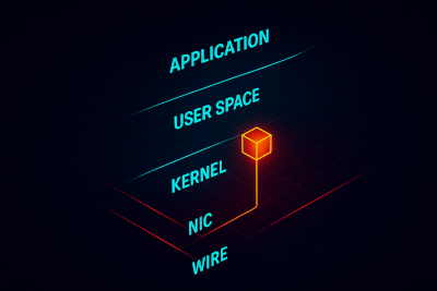
The Journey of a Packet

When a network packet arrives, it takes a long journey before reaching the application code. Let's trace that path.

1. The Wire → NIC

The packet arrives as electrical signals on the wire. The NIC's physical layer decodes these signals into bits, assembles them into frames, and validates checksums.

2. NIC → Memory

The NIC uses Direct Memory Access (DMA) to copy the packet directly into RAM without involving the CPU. The packet lands in a ring buffer (a circular queue of pre-allocated memory).

3. Interrupt → Kernel

Once the packet is in memory, the NIC raises a hardware interrupt to notify the kernel. The CPU stops what it's doing, saves its current state, and jumps to the interrupt handler.

This is expensive, so modern systems use several techniques to reduce interrupt overhead:

• Interrupt coalescing: batch multiple packets into one interrupt
• NAPI (New API) on Linux: poll for packets instead of interrupt-per-packet
• Busy polling: application constantly checks for new packets (kernel bypass)

4. Kernel Processing

The kernel's network stack processes the packet:

• Validates IP and TCP/UDP headers
• Updates connection state
• Applies firewall rules
• Copies the packet data to a socket buffer

5. Socket Buffer → Application

The application calls a syscall like recv() or read() to get the data. This triggers a user-kernel transition:

1. CPU switches from user mode to kernel mode
2. Kernel checks the socket buffer
3. Copies data from kernel space to user space
4. CPU switches back to user mode

If the data isn't ready yet, the thread sleeps until the kernel wakes it up, adding scheduling latency.

6. User Space → Application's Code

Finally! The data is in the application's memory. But we're not done yet, the application code might:

• Deserialize the message (parse binary/JSON/protobuf)
• Validate and process business logic
• Possibly allocate memory, acquire locks, or make other syscalls
• Send a response back down the stack

---

Latency Breakdown

Exact numbers vary by hardware, kernel tuning, NIC, CPU architecture, and runtime.

Layer	What Happens	Typical Range
NIC → DMA → RAM	NIC decodes frames, DMA copies into a ring buffer	0.5–5 µs
Interrupt Path	CPU handles interrupt, schedules NAPI or ISR	2–20 µs
Kernel Network Stack	IP/TCP parsing, state updates, socket buffer work	5–50 µs
Syscall Boundary	User→kernel→user mode switches + copy	0.2–5 µs
Scheduling Delay	Thread sleeps and wakes (if not busy polling)	5–100+ µs
User-Space Processing	Deserialize → parse → logic → locks → allocations	µs → ms
GC / Runtime Pauses	Python/Go/Java GC, JIT warmup, scheduler overhead	100 µs → 10+ ms

---

With the hardware and kernel path accounted for, the remaining latency comes from the runtime and language layer.

---

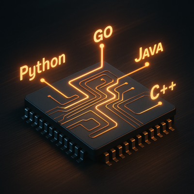
The Cost of Abstraction

The latency stack above assumes a low-level, close-to-the-metal language like C or C++. But most software is built with higher-level languages and frameworks. What's the cost?

Runtime Overheads

The choice of language and runtime has enormous implications:

Python:

• Interpreted, dynamically typed
• Global Interpreter Lock (GIL) serializes execution
• Garbage collection pauses: typically 0.1–10 ms, spikes to 50+ ms under heavy churn
• Impact: Adds milliseconds of latency per operation, unsuitable for microsecond-level work

Go:

• Compiled, but with runtime scheduler and GC
• Goroutine scheduling: ~200 ns–2 µs overhead per switch
• GC pauses: mostly <100 µs, occasional spikes ~1 ms
• Impact: Excellent for millisecond-range services

Java:

• JIT compilation warms up over time
• Modern GCs (ZGC, Shenandoah) target <1ms pauses
• JVM method dispatch / object allocation overhead: tens of µs per call in hot paths
• Impact: Viable for low-millisecond latency targets with tuning

C++:

• Direct memory control, no GC
• Zero-cost abstractions (templates, inline functions)
• Impact: The standard for <100 µs, even <10 µs targets when tuned

Regardless of language choice, the fundamental levers of low-latency design remain the same.

---

Optimization Techniques

Hitting microsecond-level latency targets is about removing friction at every layer of the stack. The techniques below form the foundation of most high-performance systems:

1. Kernel bypass: cut out syscalls and context switches
2. Zero-copy I/O: write directly to NIC buffers, skip unnecessary memory copies
3. Lock-free data structures: avoid waiting on shared state
4. Cache locality: keep hot data in L1/L2 cache
5. CPU pinning: dedicate cores to critical threads
6. Memory pre-allocation: allocate once, reuse forever in the hot path
7. Branch prediction: structure code to maximize CPU prediction rate

These topics will be covered in later articles in this series

---

Conclusion

Latency is the sum of every operation between stimulus and response. Every copy, every context switch, every syscall contributes to the total. Recognizing these hidden costs is the first step toward sound trade-offs.